本文章为https://llsf9.github.io/2023/07/17/geo-estimation/
图片处理
from PIL import Imagefrom utils import * from ImgProcess import * from model import * from visualize import *import numpy as npimage = Image.open ("/home/aiwen/GeoExplain/resources/images/im2gps/97344248_30a4521091_32_77325609@N00.jpg" ) img_array = np.array(image) im_bgr = cv2.cvtColor(img_array, cv2.COLOR_RGB2BGR) intImg = cv2.resize(im_bgr, (256 , 256 )) floatImg = np.float32(intImg) / 255 varImg = preprocess_image(floatImg) gussianBlur, medianBlur, mixBlur = blurImg(intImg, floatImg) varBlur = preprocess_image(medianBlur)
由于源代码是通过导入Dataset类进行运算的,但是我们的需求是只有一张图
因此提取出来内部的部分代码进行个性化设置
from classification.train_base import MultiPartitioningClassifierimg = varImg img_reshape = torch.reshape(img, (1 , img.size(0 ), img.size(1 ), img.size(2 ), img.size(3 ))) data = [img_reshape, {"img_id" :"0" , "img_path" : "None" }] if torch.cuda.is_available(): data[0 ] = data[0 ].cuda() images, meta_batch = data cur_batch_size = images.shape[0 ] ncrops = images.shape[1 ] images_re = torch.reshape(images, (cur_batch_size * ncrops, *images.shape[2 :]))
模型细节 导入模型
checkpoint="../models/base_M/epoch=014-val_loss=18.4833.ckpt" hparams="base_M/hparams.yaml" model = MultiPartitioningClassifier.load_from_checkpoint( checkpoint_path=str (checkpoint), hparams_file=str (hparams), map_location=None , ) model.eval () if torch.cuda.is_available(): model.cuda()
先来看一下网络的前传播的过程
def forward (self, x ): fv = self.model(x) yhats = [self.classifier[i](fv) for i in range (len (self.partitionings))] return yhats
先利用已经训练好的resnet50提取图片的情报
使用作者自己训练的分层classifier进行全连接
其次看对base model resnet50进行了哪些修改。可以看出去掉了最后两层:池化层和全连接层。由于我们接下来要传入classifier,因此还要导出最后的output的feature数。
def build_base_model (arch: str ): model = torchvision.models.__dict__[arch](pretrained=True ) elif "resne" in arch: nfeatures = model.fc.in_features model = torch.nn.Sequential(*list (model.children())[:-2 ]) else : raise NotImplementedError model.avgpool = torch.nn.AdaptiveAvgPool2d(1 ) model.flatten = torch.nn.Flatten(start_dim=1 ) return model, nfeatures
最后是classifier的网络模型,其实就是最简单的全连接层。但是注意这里的输出特征数量是不一样的,取决于len(partitionings)。这里的partitionings属于Partitioning()类。里面的len定义等同于包含的classes数量。而classes又是从外部的csv读取到的。
因此这里的不同层级的class其实已经在外部定义好了,而这里就是根据不同层级的分类数创建不同的全连接层。
classifier = torch.nn.ModuleList( [ torch.nn.Linear(nfeatures, len (self.partitionings[i])) for i in range (len (self.partitionings)) ] )
输出结果 首先生成三个层级的分类器的softmax结果
yhats = model.forward(images_re) yhats = [torch.nn.functional.softmax(yhat, dim=1 ) for yhat in yhats] [tensor([[1.4847e-09 , 2.4911e-09 , 3.7824e-09 , ..., 7.4934e-10 , 2.8366e-08 , 1.9100e-09 ]], device='cuda:0' , grad_fn=<SoftmaxBackward>), tensor([[1.1316e-10 , 2.3532e-09 , 6.3773e-09 , ..., 3.7855e-10 , 3.1215e-09 , 7.5141e-10 ]], device='cuda:0' , grad_fn=<SoftmaxBackward>), tensor([[7.8750e-11 , 4.5912e-09 , 1.2835e-08 , ..., 4.3819e-09 , 2.0498e-08 , 2.2749e-09 ]], device='cuda:0' , grad_fn=<SoftmaxBackward>)]
依旧是因为只有一张图片的原因,以下代码不产生任何变化
yhats = [ torch.reshape(yhat, (cur_batch_size, ncrops, *list (yhat.shape[1 :]))) for yhat in yhats ] yhats = [torch.max (yhat, dim=1 )[0 ] for yhat in yhats]
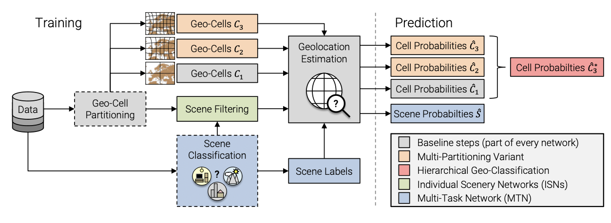
层级分类 终于到了大部头层级分类,英文名为hierarchical classification。最先由YOLO9000进行了使用。
在进行分类问题时如果只进行单一的评测标准是很不合理的。人类思考时其实也是一样的,比如判断某张照片的位置信息时我们的考虑顺序是:
有成片樱花树:大概率在日本
行人们穿的相当时尚:大概率在东京
沿着河川:大概率在目黑川
在不同的层级,我们的判断标准和关注点会有所不同。这样的多层级分类会让我们的判断更为精确。
本文的作者使用类似的思想,对国家,区级和街道进行三级分类。这有点像是个树状结构,街道只能属于一个区级和国家(叶子节点),而国家能有多个区级和街道(父节点)。最终概率的计算方式是同个枝干上的概率相乘。
首先根据上一节的输出内容,我们得到了每个层级分类器的结果。但是这时候每个节点互相不认识,不知道哪个和哪个连接。作者引入了一个12893*3的矩阵。由于一共有12893个叶子结点且相互独立,因此用这个作为标准,构建了属于每个叶子结点的枝干的class。
这个矩阵大致为这样。可以看出来最后一列的叶子结点是无重复且按顺序排列的。
array([[ 0 , 0 , 0 ], [ 1 , 1 , 1 ], [ 2 , 2 , 2 ], ..., [ 948 , 1110 , 12890 ], [ 1608 , 2250 , 12891 ], [ 709 , 799 , 12892 ]], dtype=int32)
hierarchy_logits = torch.stack( [yhat[:, model.hierarchy.M[:, i]] for i, yhat in enumerate (yhats)], dim=-1 , ) hierarchy_preds = torch.prod(hierarchy_logits, dim=-1 )
利用这个矩阵,我们对yhats进行重新构建,使之变成了均为12893长的数列。最后进行乘积计算出最终概率。